RESOURCES
OBJECTIVES & QUESTIONS
Introduction & Definitions
What is a measurement and a measurand?
What are static and dynamic measurements?
Measurement
- The 'input' (x), or physical quantity being measured, does not change over time and is therefore said to be 'steady'
- The output (y) can generally be given as a factor (K) of the input, where K is the static sensitivity of the system:
y = Kx
Measurement
- The 'input' (x) or physical quantity being measured, changes over time (t) and is therefore said to be 'unsteady'
- The output (y), as a function of time y(t) and can generally be given as a factor (K) of the input as function of time:
y(t) = Kx(t)
- Mathematically, if we let f(t) be the input to the system as a function of time and y(t) be the output, then the relationship between them is
Measurement Systems
What are the components of a measurement system?
- Produces a physical or chemical change in response to variations in the measured parameter (chemical, electrical or physical)
- Converts a signal into a useful and meaningful value
- Transducer
- 'Conditions' the signal output of the sensor into a signal suitable for the next stage of operation - mostly through conversion of a physical quantity into an electrical form
- Some overlap occurs with signal processing
- Analogue-to-digital convertors (ADC)
- Resistance circuits (e.g. Wheatstone bridge)
- Filters
- Amplifiers
- Isolators
- 'Processes' the signal through modification, enhancement and analysis
- Some overlap occurs with signal conditioning
- Analogue-to-digital convertors (ADC)
- Resistance circuits (e.g. Wheatstone bridge)
- Filters
- Amplifiers
- Isolators
- Provide an interface between the processed output signal and the clinician
- Presents graphical or numerical data, often in real-time, with storage and alarm systems
- Monitor screen
- Alarm system
- Data Processor
- Data Storage
Sources of Error
What can cause errors in a measurement?
- When discussing measurement systems it is important to be aware of potential sources of error
- These may result from:
- Error that results from 'any action or lack there of that leads to exceeding the tolerances of the conditions required for the normal functioning of the measuring system with which the human interacts' Types of human error include:
- Action errors:
- Slips – a frequently performed action is done wrong or is carried out on the wrong object
- Lapses – a step is forgotten
- Thinking errors:
- Rule-based mistakes – a good rule/method is applied in the wrong way or a bad rule is followed (when rules/procedures are available)
- Knowledge-based mistakes – applying incorrect logic, resources, or lacking experience in a situation where no rules are available
- Action errors:
- Error that is predictable and are secondary to the shortcomings of the measurement system itself
- Types of systematic error include:
- Environmental errors - the surroundings cause problems with the measurement system
- Instrumental errors - the measuring instrument itself is flawed and causes consistent inaccuracies
- Theoretical errors - the measurement procedure is flawed creating inaccuracies
- Error that is uncontrollable and unpredictable and follows a Gaussian normal distribution - can be subjected to statistical analysis to reduce error
Static Performance Characteristics
What are static measurements?
- The ‘input’ (x), or physical quantity being measured, does not change over time and is therefore said to be ‘steady’
- The output (y) can generally be given as a factor (K) of the input, where K is the static sensitivity of the system:
y = Kx
- Static characteristics are concerned only with the steady-state reading that a measurement system settles down to
What are the static characteristics that define the performance of a measurement system?
The static performance of a measurement system can be defined by:
- Accuracy
- Precision
- Linearity
- Hysteresis
- Drift
- Sensitivity
- Span
- Range
- Resolution
What are the ‘accuracy’ and ‘precision’ of a measurement system?
- The ability of a measurement device to match the true value of the quantity being measured
- It is often quoted as a % and can be calculated by the formula:
Accuracy = [(input - output) / input] x 100
- The degree to which further measurements will show the same or similar results
- In the analogy of shooting arrows at a target:
- Accuracy represents how close the arrow was to the bullseye
- Precision represents how tightly packed a cluster of arrows are once fired
- The ideal measurement device would be accurate and precise, with all repeat measurements close to each other and the average is close to the true value
How can the ‘accuracy’ and ‘precision’ of a measurement system be graphically represented?
- A straight line passing through the origin represents the true value for a line y = x
- Every measured value is plotted to exactly match the line of best fit (precision) which exactly matches the line of true value (accuracy)
- The concentric rings represent input with the true value at the center
- The location of the measured values average the point exactly at the center of the concentric rings (accuracy) and are closely packed together (precision)
- A straight line passing through the origin represents the true value for a line y = x
- Every measured value is plotted so that it lies away from the line representing the true value (imprecision) but so that the line of best fit matches the line of true value (accuracy)
- The concentric rings represent input with the true value at the center
- The location of the measured values average the point exactly at the center of the concentric rings (accuracy) but are loosely packed around the target (imprecision)
- A straight line passing through the origin represents the true value for a line y = x
- Every measured value is plotted to exactly match the line of best fit (precision) but the line of best fit lies away from the line representing the true value (inaccuracy)
- The concentric rings represent input with the true value at the center
- The location of the measured values average a point away from the center of the circle representing the true value (inaccuracy) but are closely packed together (precision)
- A straight line passing through the origin represents the true value for a line y = x
- Every measured value is plotted so that it lies away from the line representing the true value (imprecision) and the line of best fit lies away from the line representing the true value (inaccuracy)
- The concentric rings represent input with the true value at the center
- The location of the measured values average a point away from the center of the circle representing the true value (inaccuracy) and are loosely packed around the target (imprecision)
What is ‘linearity’ of a measurement system?
- Describes a measure of how well the measured value represents the true value over the full range of the system - can be considered a graphical display of accuracy
- Can be expressed as the maximum difference between the displayed and actual value, or this difference as a percentage of the maximum output
- Non-linearity can explain the limitations of calibration and importance of calibrating to increasing degrees
What is the ‘drift’ of a measurement system?
- A measure of the degree to which the measured value changes over time
- It is usually caused by temperature changes or unstable components in the system.
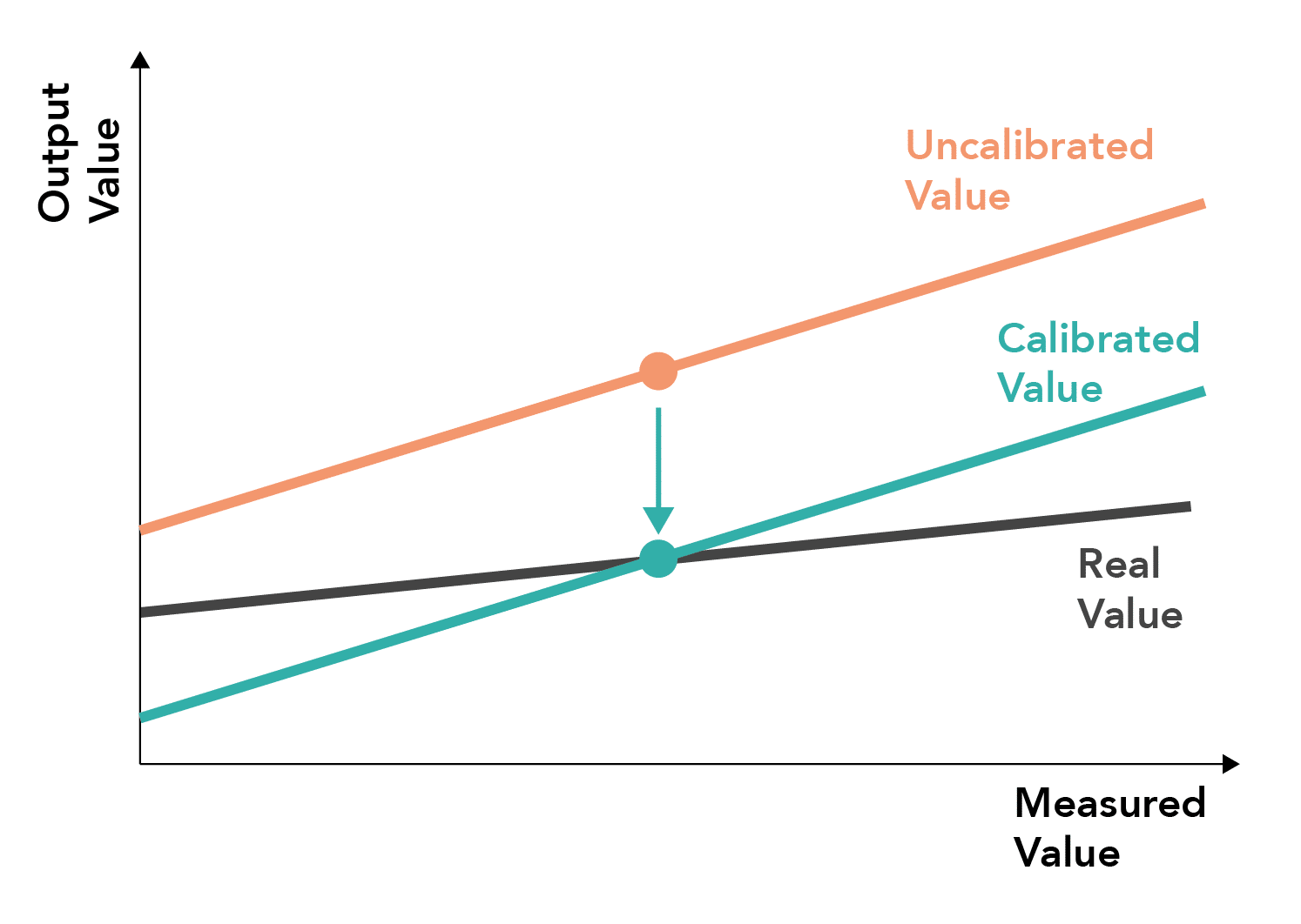
- Can take two forms - offset and gain
- A measure of the degree to which the measured value changes over time
- It is usually caused by temperature changes or unstable components in the system.
- Can take two forms - offset and gain
- A fixed deviation from the true value occurs at all points in the measured range
- Can be corrected by one-point calibration (zeroing)
- The deviation from the true value increases progressively as the upper range is approached
- Can be corrected by two-point-calibration
What is ‘hysteresis’ in a measurement system?
- The phenomenon of the difference between the measured value and the true value depending upon whether the true value is increasing or decreasing
- The graph of true value versus displayed value will have two lines: one for the true value increasing and one for it decreasing
- Causes of hysteresis may include loss of energy as friction or heat with stretching and relaxing of materials (e.g. in pressure transducers) or residual charge in electrical components
What is the span and range of a measurement system?
- The specification of a measurement system in terms of the upper and lower signal values for both input and outputs
- The interval between the upper and lower limits within which a measurement system is designed to operate
What is the resolution and sensitivity of a measurement system?
- Defines how small a change is required in the input to result in a change in the output
- Expressed as the smallest change of value of the measurand that results in a perceptible response change in device output
- Defines the how small a unit change of measurement the system is able to display
Dynamic Performance Characteristics
What is dynamic measurement?
- The ‘input’ (x) or physical quantity being measured, changes over time (t) and is therefore said to be ‘unsteady’
- The output (y), as a function of time y(t) and can generally be given as a factor (K) of the input as a function of time
- Mathematically, if we let f(t) be the input to the system as a function of time and y(t) be the output, then the relationship between them is
y(t) = Kx(t)
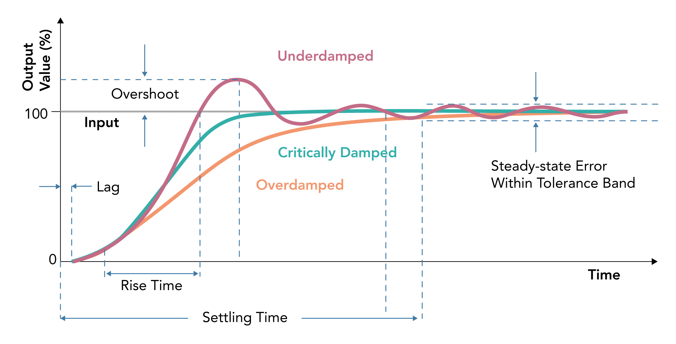
- Dynamic characteristics describe the behaviour of a measurement system between the time a measured quantity changes value and the system obtains a steady output in response
Which characteristics define the performance of dynamic measurement systems?
- The rapidity with which a measurement system responds to changes in the measured quantity.
- The time required by instrument or system to settle to its final steady position after the application of the input
- Final steady position is usually taken as a percentage of the quantity being measured (between 90-99% depending on the system)
- The time taken for the output measurement to increase from 10%–90% of the final value
- The maximum amount by which a moving system moves beyond the steady state position following the application of an input
- Overshoot is due to mass and inertia of a system
- The delay in the response of a measurement system to changes in the measured quantity
- The degree to which a measurement system indicates changes in the measurand quantity without dynamic error
- The difference between the true value of the quantity changing with time & the value indicated by the measurement system if no static error is assumed
Which standard input signals can measurement systems be tested with?
- Measurement systems receive many different kinds of input signals
- Several standards input signals are used for studying the dynamic responses of measurement systems:
- A sudden change in the measurand at time t = 0
- It is used to measure the time response of a system known as the step response
- A sudden spike in the measurand, at some time t
- Provides an alternative way of measuring a time response of a system
- A linear increase in the measurand, starting at time t = 0
- Provides an alternative way of measuring a time response of a system
- A periodic sine wave of a specific frequency and amplitude
- Provides a way to measure the frequency response of a system
What response behaviours can dynamic measurement systems display?
- Measurement systems respond differently to inputs due to their inherent properties such as resistance, capacitance, mass and dead time.
- The dynamic response of an instrument is typically described as either zero, first, or second-order:
- The order of an ideal dynamic system is zero but this does exist in clinical practice
- Most clinical measurement systems behave as either first-order or second-order dynamic systems
- Each order can be modelled by using differential equations of increasing complexity
- The displayed value tracks the measured value exactly
- The system is characterised as having:
- No inertia
- No damping
- The displayed value moves towards the true value exponentially
- The system is characterised as having:
- Time-dependent storage or dissipative ability
- No inertia
- The displayed value oscillate around the true value before coming to steady-state
- The system is characterised as having:
- Time-dependent storage or dissipative ability
- Time- dependent inertia
- Mathematically, the output from the system y(t) is given as a factor (K) of the input as function of time
- Introduces a new variable which describes the behaviour of a first order system:
- Time constant (Τ): the time constant of the exponential process
- Introduces two new variables which describe the behaviour of a second order system:
- Damping ratio (ζ): a dimensionless parameter which describes how oscillations within a system can decay once a disturbance occurs
- Undamped natural or angular frequency (ω): the frequency at which the system would oscillate in the absence of damping
- Does not truly exist in clinical measurement
- Most closely demonstrated by a potentiometer
- Demonstrated by a liquid expansion thermometer - gradually warm up from room temperature to the patient’s body temperature
- Demonstrated by a pressure transducer measuring arterial pressure waveforms, which are affected by resonance and damping in the system
Which factors influence the response of a second-order system to an input signal?
- As described previously, the ordinary differential equation used to describe a second-order measurement system introduces two new variables that describe the behaviour of the system:
- The frequency at which a system tends to oscillate in the absence of damping when caused to move or supplied with energy
- It is described in hertz (Hz)
- A dimensionless parameter which describes how oscillations within a system can decay once a disturbance occurs
- As it is a dimensionless parameter it is described without units
What is resonance?
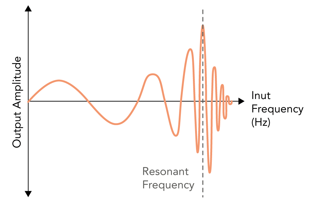
The tendency of a system to oscillate with increased amplitude that occurs when a sinusoidal input or force is applied, that is equal or close to the natural frequency of the system on which it acts
- Every material has a frequency at which it freely oscillates, known as the natural frequency
- When a sinusoidal input signal of a similar frequency is applied to the system it causes the system to oscillate at its maximum amplitude
- Can be represented on a graph of amplitude against input frequency
- As the frequency increases towards the natural frequency the amplitude increases in size
- It reaches its peak at the natural frequency of the system
- As the frequency increases further the amplitude decreases again
- The classic examples of resonance often given are:
Why does resonance occur?
- Resonance occurs when the frequency of an applied force to an oscillating system (driving frequency) is equal to its natural frequency
- The mathematics to describe this are complex but can be best appreciated by considering a child being pushed on a swing:
- The child and swing have a fixed natural frequency
- Every time the child is pushed, energy is added to the system
- When the timing of the push (driving frequency) matches exactly the natural frequency of the swing:
- Every push will be at the time of the child moving forward
- All energy inputted works to increase the height of the swing (and thus increase the amplitude of the system)
- Results in energy being added most efficiently
- When the timing of the push (driving frequency) does not match the natural frequency of the swing:
- Some pushes will be timed when the child is swinging forward but some will be timed when the child is swinging backwards
- Results in some energy being used to resist movement of the swing (and thus decrease the amplitude of the system)
- Thus, energy is added to the system inefficiently
How can you avoid resonance?
- To avoid resonance, the natural frequency of a system must differ from the input frequency
- When considering the input frequency it is essential to understand that any non-sinusoidal wave can be deconstructed into a series of harmonics through Fourier’s analysis:
- Each harmonic has increasing frequency and decreasing amplitude
- In general, to avoid resonance, it is vital to ensure that the natural frequency of a system is greater than the 8th harmonic of the input system:
- An invasive arterial blood pressure trace is assumed to have a maximum fundamental frequency of 3 Hz (equivalent to a heart rate of 180 bpm)
- The natural frequency of the measurement system must therefore have a natural frequency of >24Hz (above the frequency of the 8th harmonic) to avoid resonance
- The equation below determines the natural frequency of a system, where k is stiffness and m is mass.
- In practice, using invasive blood pressure monitoring as an example, the natural frequency of a system can be manipulated by changing the
- Stiffness of the system: radius of tubing, elasticity of tubing material
- Mass of the system: length of tubing, density of fluid
What is damping?
The tendency of a system to resist oscillation
- A decrease in the amplitude of an oscillation as a result of energy loss from a
system owing to frictional or other resistive forces. - A degree of damping is desirable and necessary for accurate measurement, but too
much damping is problematic. - The terminology should be considered in the context of a measuring system that is attempting to respond to an instantaneous change in the measured value – this is akin to the situation in which you suddenly stop flushing an arterial line while watching the arterial trace on the theatre monitor
How does the damping coefficient of a system affect the response to an input?
- The effect of the damping ratio on a system is best demonstrated by viewing the response of a system to a step input
(Damping Coefficient (ζ) = 0)
- A theoretical situation in which the system oscillates in response to a step change in the input value and the amplitude of the oscillations does not diminish with time;
- The system is un-damped because the output value continues to oscillate around the baseline after the input value has changed
- The amplitude of these oscillations would remain constant, as shown, if no energy was lost to the surroundings. This situation is, therefore, theoretical as energy is inevitably lost, even in optimal conditions such as a vacuum
(Damping Coefficient (ζ) = 0.64-0.71)
- The most suitable combination of a rapid response to a change in the input value, with minimal overshoot
- The response is fairly rapid with no more than two oscillations around the baseline before attaining the new value
- This is the level of damping that is desirable in modern measuring systems
(Damping Coefficient (ζ) = 1)
- That degree of damping which allows the most rapid attainment of a new input value combined with no overshoot in the measured response
- The response is still blunted, but any faster response would involve overshoot of the baseline
- Critical damping is still too much for a rapidly responding measurement device
(Damping Coefficient (ζ) > 1)
- The system response is overly blunted in response to a step change in the input value, leading to inaccuracy
- This time the curve falls extremely slowly towards the new value
- Given enough time, it will reach the baseline with no overshoot but clearly this type of response is unsuitable for measurement of a rapidly changing variable such as blood pressure
Why is resonance and damping important in clinical measurement?
- Many measured inputs are periodic in nature (e.g. arterial pressure waveform), meaning resonance and damping become important factors in the measurement systems
- Over or under-damping can lead to inaccurate clinical measurement
- Measurement systems are carefully designed and ‘tuned’ in terms of natural frequency and damping ratio to manage the specific periodic input signal
Calibration Fundamentals
What is calibration?
- Defined by the ‘International Organization for Standardization’ as:
The set of operations that establish, under specified conditions, the relationship between values indicated by a measuring instrument, a measuring system or values represented by a material measure, and the corresponding known values of a measurand
- Calibration checks for accuracy and linearity by comparing measurements with known values (standards) at set points
- Thus, it ensures that the measured value equates to the input value at these points
What is a standard?
A material measure or physical property that defines or reproduces the unit of measurement of a base or derived quantity
- The standard should be of the same nature as the measurand
- It should generally be traceable to an international or international standard or acceptable alternative
- The most important standards are the fundamental and derived SI units (System International)
Why is calibration important?
- Used to ensure reliability in a measurement system:
- Confirm accuracy and precision of measurement
- Remove the effects of drift (offset and gradient)
- These variations in measurement systems may occur due to:
- Manufacturing variations
- Differing system designs
- Change in response to environmental parameters (heat, cold, humidity)
- Ageing of systems over time
Calibration Types
What is one-point calibration?
- The simplest form of calibration
- Involves measuring a single point against a standard and correcting for sensor offset against this point
- The offset correction is then applied in a constant manner to all the measurements returned by the instrument
- Useful if a system exhibits offset drift and linearity
- Often known as zero-point calibration or “zeroing”
What are the problems with one-point calibration?
- Only ensures a single point is correct against the standard but cannot correct for incorrect linear gradients
- May result in inaccurate measurements at the extreme of the measurement system range
What is two-point calibration?
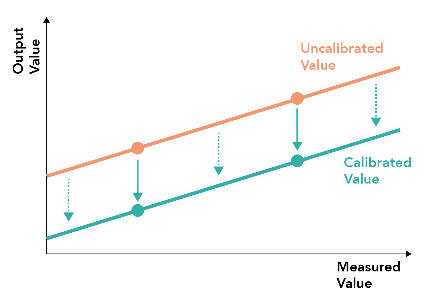
- Involves measuring two points against a standard and correcting for sensor offset against these points
- The correction can then be applied to all measurements using a line of best fit between the points
- Two points lying within the physiological span of measurements should ideally be used, generally at the extremes of the measurement spectrum
Useful if a linear system exhibits both offset and gradient drift
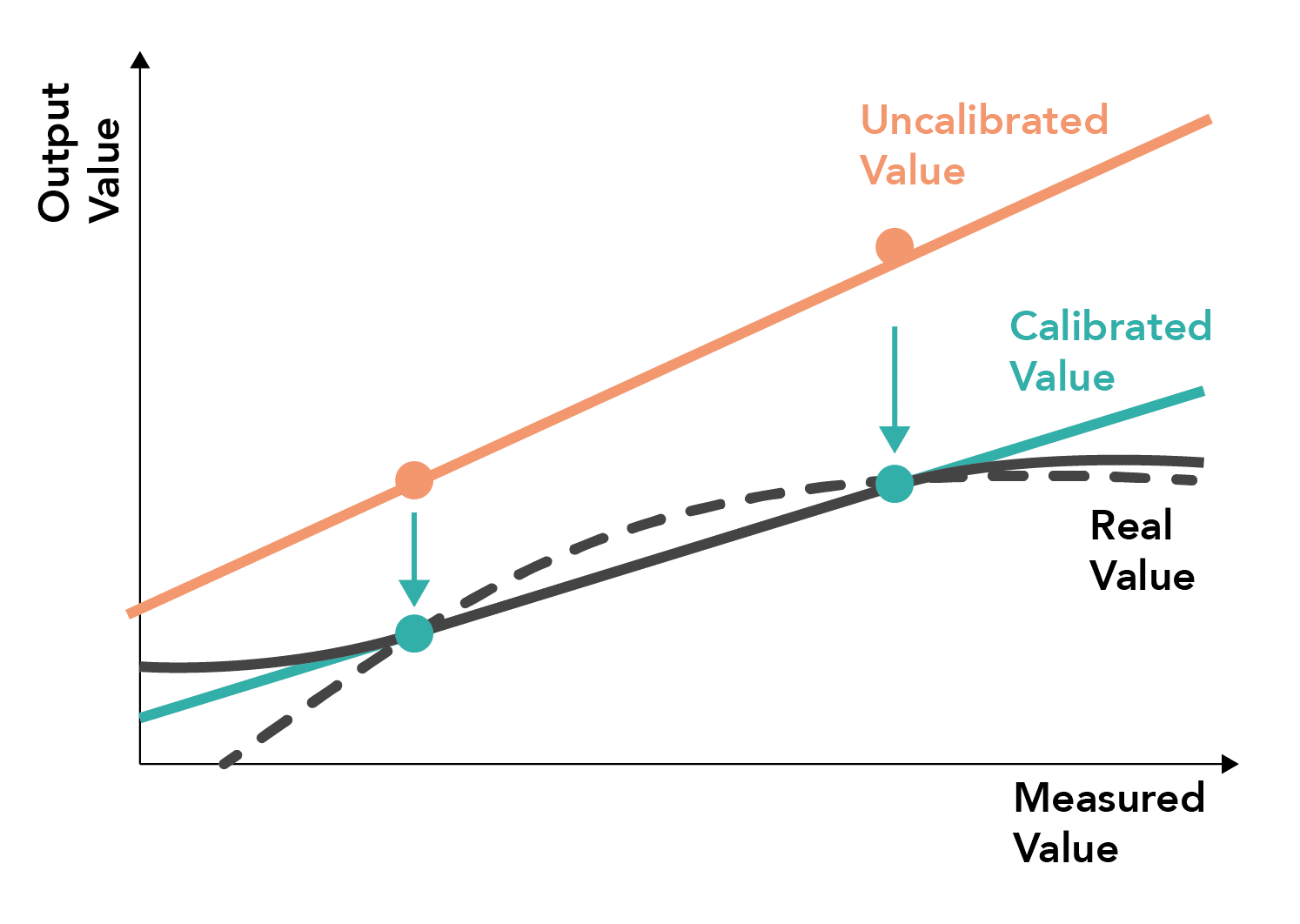
What are the problems with two-point calibration?
- Useful for correction of linear systems correcting for both linear and gradient drift between calibrated points
- May result in inaccurate measurements when the system behaves in a non-linear manner (dashed line) or the measurement system changes behaviour outside the range of the calibrated points (solid line)
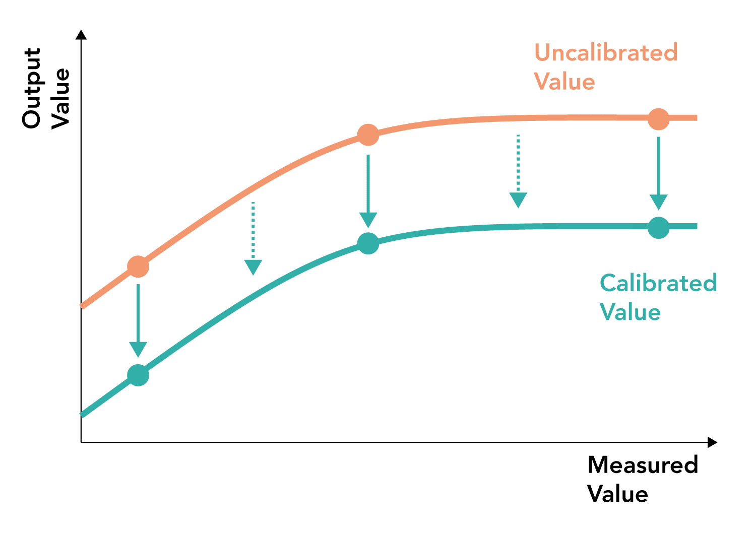
What is multi-point calibration?
- The most accurate form of calibration
- Involves measuring multiple points against a standard and correcting for sensor offset against these points
- The correction can then be applied to all measurements using a line of best fit between the points
- Can be useful when a measurement system behaves in a non-linear manner
- Ideally points should be selected at the extremes and across the range of the measurement spectrum
Measurement Principles in Invasive Blood Pressure Monitoring


